katrinteubner

geographische lage dieses städtischen sees und benachbarter seen

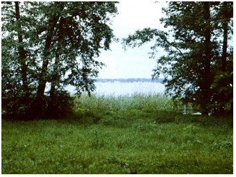
Großer Müggelsee, 1995:
Blick vom Südufer über den flachen See. Viele Segelboote sind an diesem Sommertag auf dem Wasser zu sehen. Der Große Müggelsee (52°26’5.56''N, 13°38’6.2''E) befindet sich in Berlin (Deutschland) und liegt 45 m über dem Meeresspiegel. Es ist ein kleiner See mit einem Volumen von 36 m³ und einer nahezu kreisförmigen Fläche von 7 km². Die maximale Tiefe des Sees beträgt nur 7,7 m. Die thermische Umwälzung dieses flachen Sees (vertikale Durchmischung) ist daher sehr häufig im Jahr und wird als polymiktisch bezeichnet. Die mittlere theoretische Verweilzeit des Wassers im Seebecken beträgt nur 67 Tage. Sie ist damit deutlich kürzer als die Verweilzeit in großen, tiefen Seen, wie sie beispielsweise für die alpine Region auf dieser Website beschrieben wird (1-7 Jahre Verweilzeit bzw. engl. „retention time“, siehe z.B. Ammersee S, Attersee S, Mondsee S und Traunsee S). Ein weiterer flacher See in der unmittelbaren Nachbarschaft vom Großen Müggelsee, ist der Lange See (52°23’54''N, 13°38’2.96''E) . Dieser See hat eine ausgeprägt längliche Beckenform (siehe Foto vom Langen See vom Müggelturm hinunter, unten im Text). Die Verweilzeit des Wassers im Langen See ist noch viel kürzer als im Großen Müggelsee. Sie beträgt nämlich im Mittel nur 4.13 Tage (die mittlere Retentionszeit beider Seen bezieht sich auf die Jahre 1992 und 1993; Kohl et al. 1995, Tabelle 1 in Teubner et al. 1999 R, Tabelle 1 in Teubner & Dokulil 2002 R). Die seenartigen Aufweitungen von Flüssen im nördlichen Tiefland Mitteleuropas sind einerseits weit entfernt von einem „typischen“ See, aber stellen andererseits auch nicht wirklich „nur“ einen Fluss dar. Weitere Beispiele solcher Gewässer sind der Seddinsee (52°23’4.7''N, 13°40’53''E) und der Flakensee (52°25’55''N, 13°45’48.7''E), die wiederum eine kurze mittlere Verweilzeit des Wassers von nur 13 bzw. 29 Tagen aufweisen (Bezug auf die Jahre 1992/1993, Verweilzeit siehe Kohl et al. 1995). Gewässer in dieser Zwischenstellung von Fluss und See, die sich durch eine mittlere theoretische Verweilzeit des Wassers von etwa 3 - 30 Tagen (bzw. bis zu etwa 70 Tagen) kennzeichnen lassen, werden als „Flußseen“ (engl. „riverine lakes“) bezeichnet. Die Gewässer, mit einer kürzeren bzw. längeren Verweildauer des Wassers bilden charakteristische Fluss- bzw. Seenökosysteme und sind dementsprechend als Flüsse bzw. Seen definiert. Flußseen sind in der Auenlandschaft der Flüsse Spree, Dahme und Havel in der Öko-Region um Berlin, d.h. in Brandenburg und Mecklenburg, weit verbreitet.

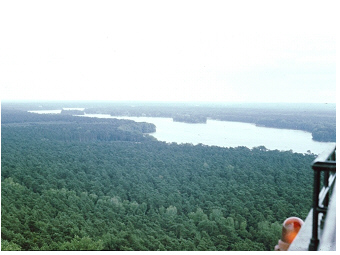
Blick vom Müggelturm hinunter auf den “Fluss-See (Flußsee)” Langer See, 1995:
Aus der Vogelperspektive ist die längliche Form des Wasserbeckens gut zu sehen. Der Lange See sieht eher wie ein Fluss als ein See aus. Die Flußseen werden im deutschen Sprachraum auch als „seen-artige Erweiterung eines Fließgewässerabschnittes“ umschrieben. Je kürzer die Verweilzeit, desto größer wird der potenzielle Einfluss des Auswaschens auf die Entwicklung der planktischen Organismen im Gewässer. Insbesondere für das Aufkommen von manchen Zooplanktonarten, die für ihre Entwicklung vom Ei bis zum erwachsenen Stadium eine Zeitspanne von mindestens 30 Tagen benötigen, muss die Verweildauer des Wassers im Becken wenigstens 30 Tage betragen. Daher kann die Strömungsgeschwindigkeit bzw. die Verweilzeit des Wassers die Qualität und die Länge der Nahrungskette im Ökosystem und damit auch die Phytoplanktonzusammensetzung beeinflussen. Die Flußseen gehen räumlich oft direkt ineinander über, sodass stark durchflossene Flußseen mit weniger stark durchflossenen Flusseen verbunden sind und letztere dann auch als Brutstätte für das Zooplankton für nachfolgende Flußseen dienen können. Außerdem bilden beruhigte Uferzonen und kleinen Uferbuchten in einem stark durchflossenen Flußsee zusätzlich Retentionsräume, die der Entwicklung von Zooplankton dienlich sind. Rädertierchen und Krebstier-Zooplankton (Cladocera und Copepoda) sind in den beiden bereits genannten Flußseen, Großer Müggelsee und Langer See (Abb. 7 in Teubner et al. 1999 R), verbreitet. Diese Zooplanktonarten entwickelten hohe Individuenzahlen in beiden Gewässern, welche durch  Massenentwicklungen von Cyanobakterien über die gesamte Vegetationsperiode 1992/1993 geprägt waren (Cyanobakterien Dominanz im Frühjahr durch Limnothrix redekei & Planktothrix agardhii, von Sommer bis in den Herbst von P. agardhii oder von Aphanizomenon flos-aquae & Microcystis spp., siehe detailliertere Angaben zum Phytoplankton im unten nachfolgenden englischen Textabschnitt und auch deutschsprachig in Teubner 1996 R). Die Phytoplankton-Verlustraten durch Zooplanktonfraß wurden über mehrere Fütterungsexperimente mit filamentösen Cyanobakterien (Planktothrix agardhii) im Frühjahr 1993 abgeschätzt. Die Verlustraten des Phytoplanktons durch Zooplanktonfraß betrugen 0,17 d^-1 für den stark durchflossenen Langen See und waren fast doppelt hoch, nämlich 0,3 d^-1 für den Großen Müggelsee, der durch eine längere, d.h. eine etwa zweimonatige Verweildauer des Wassers charakterisiert ist (Seiten 334-335 in Teubner et al. 1999 R).
Im Gegensatz zum Zooplankton entwickeln sich die Zellen des Phytoplanktons meist sehr rasch. Wie an anderer Stelle auf dieser Website detaillierter beschrieben ist, kann man davon ausgehen, dass sich die Zellen des „natürlichen Phytoplanktons“ unter sehr günstigen Wachstumsbedingungen, wie zum Beispiel im zeitigen Frühjahr, bereits innerhalb eines Tages (24 h) oder zumindest aller 2-3 Tage ein Mal teilen. Unter ungünstigen Wachstumsbedingungen für das Phytoplankton kann sich jedoch auch hier die Zellteilung und damit das Wachstum gut über einige Wochen hinauszögern. Im Gegensatz zu dem natürlichen Phytoplankton werden bei Algenkulturen die „künstlichen“ Laborbedingungen oft so gewählt, dass in etwa eine Zellteilung pro Tag „garantiert ist“.
Wie oben bereits beschrieben, werden Flußseen allgemein als recht rasch durchflossene flache Seenökosysteme beschrieben. Sie wechseln ihren Charakter nicht im Verlaufe eines Jahres. Ein natürliches Wasserbecken kann aber auch in seinem Charakter je nach Jahreszeit zwischen einem Fluss und einem See wechseln. Dieser Gewässertyp wird anhand eines riesigen subtropischen flachen Sees, dem Poyang S in der Flussebene vom Jangtsekiang S in China auf dieser Website beschrieben.

Wie manch andere flache Seen in urbanen Regionen in der Welt (siehe z.B. Alte Donau S in Österreich, Taihu S and Dianchi S in China auf dieser Website), durchlebten auch die Flußseen um Berlin große Veränderungen im Ökosystem durch erhebliche Nährstoffanreicherungen über viele Jahre. Die Nährstoffbelastung war im wesentlichen auf einen externen Phosphateintrag aus dem Einzugsgebiet zurückzuführen. Der Umkehrpunkt für die externe Nährstoffzufuhr in den Flußsenn fällt historisch mit dem Jahr des Falls der Berliner Mauer im Jahre 1989 zusammen, als sich abrupt die Wirtschaftweise grundlegend änderte und sich damit Trends umkehrten, nämlich in Richtung eines rasant abnehmenden Nährstoffeintrages und einer verringerten Verschmutzung. Die Beschreibung der Flußseen auf dieser Webseite beziehen sich auf eine Vier-Jahres-Studie von Januar 1990 bis Dezember 1993. Während jener Untersuchungszeit lag noch immer eine seen-interne nährstoffangereicherte Gewässersituation vor. Dieser Gewässerzustand ist anders als jener Zustand eines „natürlich eutrophierten Flußsees“ viele Jahrzehnte zuvor bzw. in der jetzigen Zeit.

Die drei nachfolgenden Textabschnitte besprechen, warum der Große Müggelsee limnologisch als “der perfekte See” bezeichnet werden kann; warum es in diesem Flußsee relativ einfach ist, im Frühjahr eine genaue Prognose für die Phytoplanktonentwicklung für den Sommer zu geben und warum sich die Phytoplanktonentwicklung in den Seen der Berlin-Brandenburg Region statt in vier verschiedene Jahreszeiten eigentlich nur in zwei wesentliche Jahresperioden untergliedert. 

Der perfekte See: jahreszeitlich ausgewogene Nährstoffverhältnisse sind ideal auf die saisonal wechselnden Ansprüche eines optimalen Phytoplanktonwachstums im Müggelsee eingestellt

The relative quantity of nutrient elements of phytoplankton cells grown in a natural aquatic system is not by random but within a certain narrow range. The elemental composition of phytoplankton was described by Redfield stoichiometry (1958) for the ocean, called the Redfield ratio (C:N:P=106:16:1). The validity of this ratio for other aquatic habitats, other aquatic biota and other elements (N:P:Si=16:1:17 see Harris, 1986) was extensively discussed in the following years. The main nutrient elements nitrogen, phosphorus and silicon used to build-up phytoplankton biomass, are hence not utilized by phytoplankton cells by the same amount of each element (1:1:1, see Fig.14 on page 26 in Teubner 1996 R and Fig.3 in Teubner & Dokulil 2002 R) but rather close to the molar proportion of N:P:Si=16:1:17. Nutrient ratios are often assessed by x-y-plots of individual pairs of elements, as the N:P, the Si:P and the Si:N ratio. Graphs displaying together all three nutrient elements in an x-y-z plot are of the same low information and are even trickier to visualize by the three-dimensional display. A direct way for interrelated stoichiometry between the three main nutrient elements is revealed by triple ratios displayed in trigonal plots (see method and  Fig.1 in Teubner & Dokulil 2002 R). Such ratios, as N:P:Si, have the benefit of presenting multiple resource-ratio gradients and hence provide a more synoptic view than individual ratios as N:P, Si:N and Si:P. For the reason of short turnover time, ecological lake stoichiometry is commonly NOT described by the soluble reactive phosphorus fraction (this phosphorus fraction can be utilized by algae) or dissolved inorganic nitrogen (nitrate, nitrite, ammonia), but by the total pool of all fractions of phosphorus and nitrogen. In particular, in case of rapidly recycled phosphorus, common sampling methods are not really appropriate to follow the high-resolution distribution pattern of small spatial and short temporal scales of SRP in a lake. Different from P and N, in the case of silicon the physiologically relevant fraction is the dissolved fraction of soluble reactive silicon (see different turnover times for N, P and Si in the section for lake Traunsee). The triple molar ratio TN:TP:SRSi=16:1:17 can be used as a reference point for ecological stoichiometry (Teubner & Dokulil 2002 R), called the ‘optimum ratio’, in the sense of Redfield (1958) and Harris (1986) for plankton communities. Displaying the TN:TP:SRSi ratio in trigonal graphs, an axis scaling in the proportion of 16:1:17 is most appropriate and shifts the optimum point of TN:TP:SRSi=16:1:17 graphically to the triangle centre (see below the concept of the ‘balance of TN:TP:SRSi-ratios’ in lakes, Teubner & Dokulil 2002 R). Such triangular diagrams scaled in the physiological proportion of 16:1:17 aim at synoptically presenting relative nutrient availability for both diatoms and non-siliceous algae in phytoplankton communities (Fig.15 on page 28 in Teubner 1996 R, Fig.4 in Teubner & Dokulil 2002 R, for Old Danube Fig.5 E-F in Teubner et al. 2003 R, for Traunsee Fig.5 B, C, E in Teubner 2003 R).

Commonly, a one element (i.e. TN or TP or SRSi) is seasonally invariant relative to the remaining two elements in a lake. These are lakes with ‘imbalanced nutrient ratios’ (Teubner & Dokulil 2002 R). Lakes where TN:TP:SRSi ratios fluctuated evenly around the ecological reference point of TN:TP:SRSi=16:1:17, in a cyclic pattern within a given year, are the exception rather than the rule (lakes with ‘balanced nutrient ratios’). Assuming that the optimum ratio 16:1:17 indicates average requirements of algae in the plankton communities, it is not surprising, that the lakes with balanced nutrient ratios yield the highest algal biomass in comparison with other lakes of the same trophy (see hyperthrophic lakes LANS and MUES and its inflow MUEZ: the triple nutrient ratios are shown in Fig.4A and the TP:chlorophyll-a -response in Fig.2A in Teubner & Dokulil 2002 R). The shallow lake Müggelsee with high annual phytoplankton biomass for the nutrient-rich period 1990-1993, provides an example for a lake with balanced nutrient proportions. In that study period of the early nineties, the three nutrient elements in lake Mueggelsee had a stoichiometry that suited perfectly the requirements of phytoplankton growth.

The Redfield Ocean is seen as the ‘perfect sea’ due to a balanced flow of C, N and P in and out of the biota. In the context of stoichiometric ecology, lake Grosser Mueggelsee stands for the ‘perfect lake’ (see text on page 6 in Teubner 2004) for three reasons: (i) the nutrient-resource situation, described by TN:TP:SRSi ratios (1990-1993), shifts evenly around the stoichiometric optimum of 16:1:17 within a year and (ii) the elemental ratio of biota (stoichiometry of particulate organic matter, POM, POC:PON:POP) is very close to C:N:P=106:16:1. An overlay of both seasonal patterns, TN:TP and PON:POP, mirrors the complementary relationship between external and internal stoichiometry of plankton in Grosser Mueggelsee. Such stoichiometric shift towards the limiting element seems to be a common phenomenon of individual adaptation of producer organisms and can be even recognised on an ecosystem level (more details see Teubner & Dokulil 2002 R; and  Fig.5F and text on page 1147 in Teubner et al. 2003 R).

seasonal plankton dynamics: how accurate can a ‘phytoplankton forecast’ be for lake mueggelsee?

Summer phytoplankton in nutrient-rich lake Grosser Mueggelsee was commonly dominated by the cyanobacteria Aphanizomenon flos-aquae and Microcystis spp., while alternatively in a neighboring shallow lake Langer See the cyanobacterium Planktothrix agadhii was mainly developed (study period 1990-1993). A sensitive moment for the differentiation of the plankton development to the one or the other cyanobacterial summer bloom was the time in the year (Julian day), when the total nitrogen to total phosphorus ratio, the TN:TP ratio, dropped below the critical threshold value of 16:1 (Figs. 39-40 on page 110-111 in Teubner 1996 R, Figs. 1-2 in Teubner et al. 1999 R). In addition, the phytoplankton composition at this critical moment was of decisive importance. Rapid growth of the N²-fixing A. flos-aquae was favoured at TN:TP<16:1 in both lakes, when the timing of the critical TN:TP ratio and low biomass of P. agardhii due to the clear water phase coincided. In all four years studied the lake Mueggelsee, the rapid growth of the heterocyst-forming cyanobacterium A. flos-aquae started at the time when TN:TP was equal to 16:1, even in those years when this critical ratio was delayed by several weeks. In some years, however, the spring biovolume of P. agardhii was already quite high that early in the year. In such years, P. agardhii exceeded already the biovolume of 6 mm³ L^-1 at the time when the critical TN:TP ratio was reached. The mass development of this cyanobacterium was then further continued, the summer into autumn, whereas A. flos-aquae was only present in traces during the growing season. This alternative blooming of these two cyanobacterial regimes was further associated with different planktonic diatom assemblages. A summer-autumn plankton dominated by A. flos-aquae was associated with filamentous diatoms Aulacoseira spp, while Planktothrix agardhii with Stephanodiscus hantzschii, Cyclostephanos dubius and Actinocyclus normanii.

To summarize, it seemed to be a simple story to predict in late spring what cyanobacteria in summer would grow in such eutrophied shallow lakes of short retention time. Actually, even just described for this four-year study period in the nineties, this rule of alternative blooming of cyanobacterial regimes (Teubner et al. 1999 R) was seen also for other years in these two lakes. It was somewhat of a scientific gamble in spring, to project how phytoplankton situation will evolve in the very next days with the on-set of summer. The weather forecast is common, but it seems that under such a certain circumstance, some phytoplankton forecast s work as well?! In view of aquatic science, the timing of events, e.g. the date in the year passing a certain threshold of light availability, water temperature or nutrient concentration, is commonly studied for lake ‘phenology’. Such aspects are most relevant to the study of the climate response of lakes (see Mondsee S and Ammersee S).

seasonal phytoplankton structure: the only two principal periods a year

Parsteiner See im Biosphärenreservat Schorfheide-Chorin, nördlich von Berlin, 1990:
Für diesen tiefen mesotrophen See betrug der Jahresmittelwert der Sichttiefe 4,4 m. Der Parsteiner See war einer von 11 Gewässern im Norden Deutschlands, die bei einer limnologischen Studie zur Phytoplanktonentwicklung untersucht wurden. Die mittlere Sichttiefe der beiden Flußseen Großer Müggelsee und Langer See war in dieser Studie deutlich niedriger, nämlich nur 0,9 bzw. 1,6 m (Untersuchungszeitraum 1990-1993). Beside Grosser Mueggelsee and Langer See, nine other mainly shallow lakes were studied in the nineties in the Berlin-Brandenburg region (see map in Fig.1 in Teubner 1996 R). The majority of these temperate lakes were shallow and covered trophic states from mesotrohic to hypertrophic. In the vicinity of urban area of Berlin, lake Grosser Mueggelsee and lake Flakensee and its both inflows, lake Langer See, the groundwater-seepage lake Kiessee (52°39’9.4''N, 13°22’59''E) and the dystrophic lake Krumme Lake (52°25’5.2''N, 13°41’17.39''E) were studied. Furthermore, three mesotrophic lakes in the north of Berlin, the Biosphere Reserve Schorfheide-Chorin, were included. These were two dimictic lakes Parsteiner See (52°55’48.6''N, 13°59’7.7''E) and Rosinsee (52°53’28.2''N, 13°58’27''E) with a maximum depth of 27 and 9 m respectively and one shallow, slightly dystrophic lake, Grosser Plagesee (52°53’16.8''N, 13°56’16.7'E; Table 2 in Teubner 1996 R, Table 1 in Teubner & Dokulil 2002 R, Table 1 in Teubner 1997 R).

The taxa found in the 11 water bodies, referred mainly to the cyanobacteria, diatoms (Teubner 1995 R, Teubner 1997 R) and chlorophytes. Common species during that study are illustrated by microscopical photographs (pages 57-67 in Teubner 1996 R, diatoms only on  pages  238-247 Teubner 1997 R). The individual sites were studied over 3 to 4 years from 1990-1993, which accounts for ‘34 lake-years’ (page 7 in Teubner 1996 R). The two main results of phytoplankton seasonality found for these sites are described in the following paragraphs.

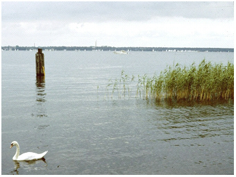
VIDEO Plauer See, Ostufer bei der Lenzer Höh', 2022:
Das klare Wasser (Teubner et al. 2020 R, 2021 R, 2022 R) verweist auf den mesotrophen Gewässerzustand dieses Sees in Mecklenburg-Vorpommern. Ein Schilfröhricht im flachen Uferbereich, im wesentlichen hier durch Phragmites australis gebildet, ist charakteristisch für die nord-deutschen Seen. Das Schilf kann sich an diesem Seeufer durch die Beschattung der Bäume jedoch nur wenig ausbreiten. The one outcome relates to the seasonal change in the size structure of phytoplankton assemblages. After spring overturn of the water body and therefore, at the time of the replenishment of nutrients from deeper water into the surface layer, mainly small short-lived forms dominate the assemblage. At this time, the so-called ‘bottom up effects’ control the phytoplankton development, that mainly small fast growing phytoplankton species become predominant. According to allometric rule (i.e. here that cell physiology depends on cell size), the fraction of small-sized cells of phytoplankton can achieve a higher photosynthetic efficiency than that of large-sized cells (see ¹⁴C measurements on phytoplankton from the alpine region: Lake Lucerne, Traunsee and Mondsee, table 2 in Teubner et al. 2001 R). The small cells are hence adjusted to low underwater light intensities. They benefit from low incoming radiation as typically found in spring. This situation early in the year usually coincides with the nutrient replenishment by overturn (mixing of the water body by wind in spring) or by external nutrient load from the catchment. The advantage of being small was found to be in accordance with their cellular pigment ratio, of having relatively high concentrations of light-harvesting chlorophyll-a but low of light-protective ß-carotene (Fig.8 in Teubner et al. 2001 R). The opposite applied for the large cells of phytoplankton assemblages. They accomplished a lower photosynthetic efficiency which was associated with a lower pigment ratio of chlorophyll-a to light-protective ß-carote. They hence indicated an adjustment to high under water light intensity. Large cell forms or colonial forms with a longer life span are rather common in summer, in particular, at the growth period immediately after a clear-water phase. This period relates therefore, primarily to a ‘top down control’, i.e. the effects by selective grazing pressure of zooplankton on phytoplankton. The dynamic of changing size structure with seasons could be illustrated by the annual time-course of the surface to volume ratio of phytoplankton (pages 79-86 in Teubner 1996 R, Teubner & Dokulil 2000 R, see also seasonal phytoplankton develpoment discussed for see Bergknappweiher S). This ratio increased from winter to spring, reaching often even an annual peak before it was when abruptly declining within few weeks (Fig.22 A-C on page 79 shows examples for lake Grosser Müggelsee and its inflow 'Müggelsee-Zufluß', and lake Langer See, in Teubner 1996 R). With the exception of the pico-phytoplankton size fraction, which is defined by a cell size smaller than 2µm and not studied here, higher ranked taxa as the Ulotrichales (needle shaped green algae), Oscillatoriales (non-colony forming trichomes of some cyanobacteria) and Pennales (needle-shaped diatoms) have exceptional high surface to biovolume ratios (Fig.23 on page 82 in Teubner 1996 R). Examples of taxa of low surface to biovolume ratios are the dinoflagellates. Large differences also can be found with a phytoplankton group. The thin trichomes of the common cyanobacteria Planktolynbya limnetica and Limnothrix redekei have a much higher surface to volume proportion than the cyanobacterial trichomes of Anabeana taxa (Fig.24 on page 83 in Teubner 1996 R) . Further within the diatoms, the pennate Nitzschia acicularis or the small centric diatoms of Cyclotella atomus or Stepahonodiscus pseudostelligera, C. parvus and C. minutulus indicate much higher surface to volume ratios than the large cells of unicellular centric diatom Actinocyclus normanii and the filamentous forms of centric diatoms, Melosira spp. (Fig.25 on page 84 in Teubner 1996 R). The annual mean values of surface to volume ratio varied among the 11 sites. These values, however, were statistically NOT significant different while the nutrient state varied largely among the water bodies (Fig.26 on page 85 in Teubner 1996 R, Table 1 in Teubner & Dokulil 2000 R). It can therefore be concluded that the surface to volume ratios of phytoplankton was not linked to the trophic state but mirrors the general pattern of intra-annual phytoplankton succession as mentioned before for the annual time courses in this paragraph.

The second pattern of phytoplankton seasonality refers to the timing of the compositional shifts within the year. This study focused on cyanobacteria and diatoms, as these phytoplankton taxa were common in the 11 studied water bodies. It could be found for the ’34 lake-years’ that the composition of winter and spring phytoplankton, on the one hand, and of summer and autumn phytoplankton on the other were statistically quite similar. Further, the winter and spring phytoplankton was statistically far different composed from those in the summer-autumn period. Therefore, significant compositional changes for both algal classes occurred concurrently two times a year only, i.e. during the transition from spring to summer and from autumn to spring (Figs.36&56 on pages 104 & 136 in Teubner 1996 R, DCA-plots of Figs.4&5 in Teubner 2000 R, see also seasonal phytoplankton develpoment discussed for see Bergknappweiher S). This reduction of seasonality from four to just two principal phytoplankton assemblages a year coincided with the seasonal pattern of the TN:TP-ratio, while those of SRSi:TN and SRSi:TP proportions varied among sites dependent from individual lake basin morphometry and the geological background (TN = total nitrogen, TP = total phosphorus, SRSi = soluble reactive silicon). The interpretation of the nutrient status by the dissolved fraction as for silicon on the on side and by the total pool as for nitrogen and phosphorus on the other, refers mainly to the different turnover time of these three nutrient elements and is in greater detail discussed for the lakes Mondsee S, Traunsee S and Old Danube S on this website.